Search algorithms for synthesizing a light-adjusting filter shape
This is part of a series exploring the design of a novel photo-exposure technique for screen printing and other light-sensitive media (cyanotypes, platinum and palladium prints, photo-chemical etching, etc). This exposure technique scans a light strip across the screen and stencil, using focusing lenses to achieve the excellent exposure characteristics of a room-sized projection lamp in the compact space of a typical light table.
Previous work first explained projection issues and sketched out the idea, and a later project demonstrated that exposure variation could be minimized sufficiently for many processes through measurement of lenses and simulation of different spacings.
A follow-on project for prototyping a scanning photo-exposure unit is creating silhouettes for minimizing variation across the cumulative exposure of a scanning strip. A silhouette filter is a flat shape placed in profile over each LED and its lens, to selectively trim specific areas of the light shape. (For example, the bat signal, used to summon the batman, is made with a bat-shaped silhouette placed over a search light.)

An ideal silhouette shape lowers the cumulative exposure variation across the strip, making the scanning technique work for more variation-sensitive processes. The 3-5% variation achieved through careful choice of spacing alone is excellent for many processes using an emulsion layer; these have variation tolerances upwards of 20%. But this level of variation does not work for more sensitive processes, like platinum print photography and cyanotypes; the artifact of the lights combining, in the form of the characteristic big-hump, little-hump pattern, will image in the print. These processes need less than 0.5% to 1% variation.
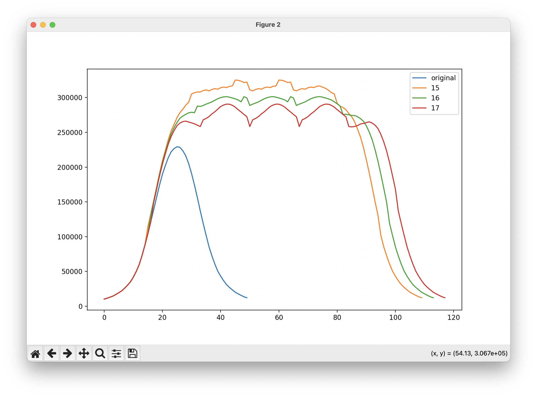 This is what a cumulative exposure looks like; an individual spot is included. Note the humps on the pattern’s plateau.
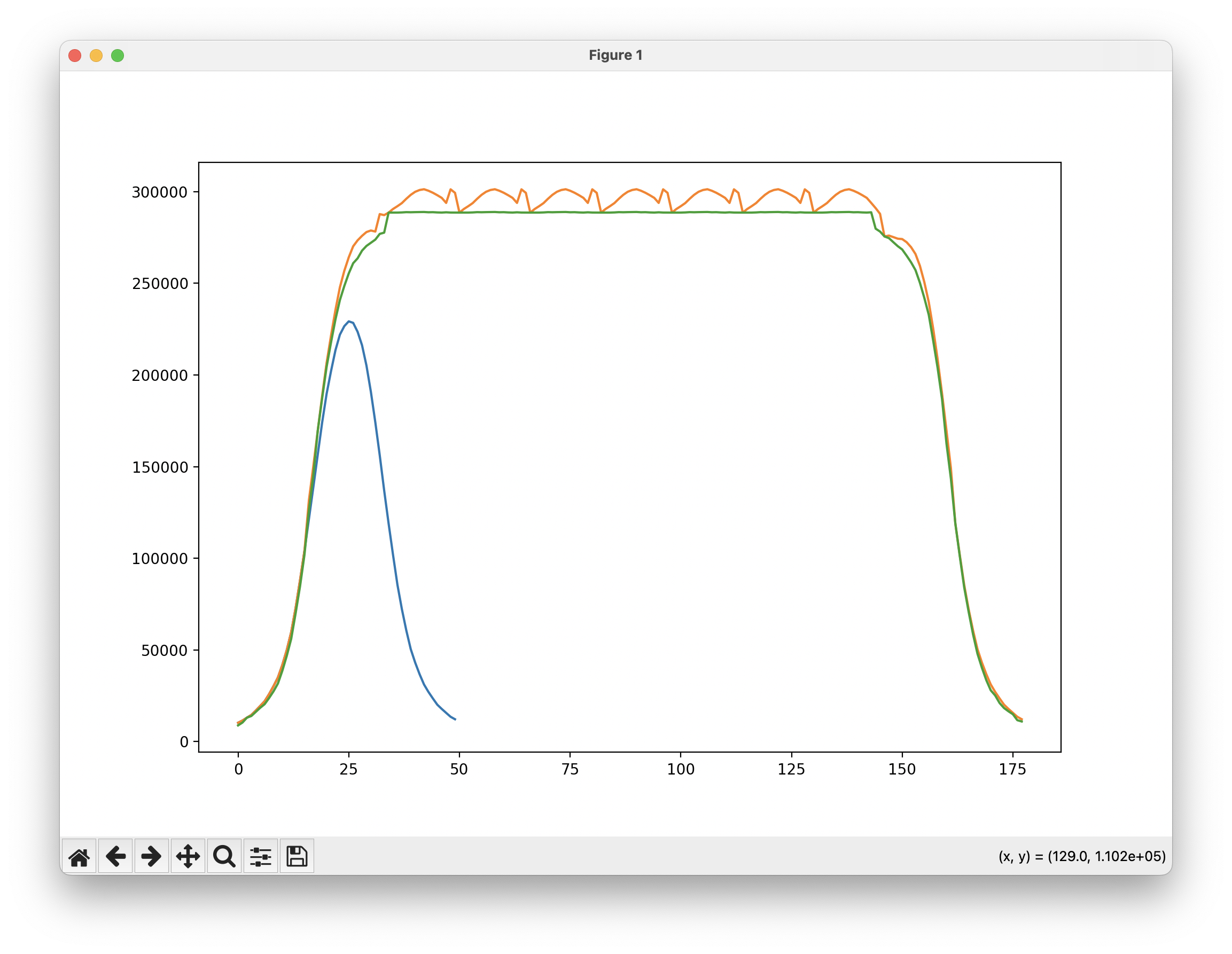 This is what the same light spot (copied a few more times) looks like (orange), compared to its profile after flattening with a silhouette filter (green). The flat plateau is ideal.
This post examines a search algorithm for synthesizing the shape of this filter, finding that a greedy algorithm using a heuristic that evaluates and maintains edge smoothness (and consequently manufacturability) can synthesize a mask that lowers the variation to under 0.5%.
Search State
Measurement and Mask
The measurement data used to find ideal spacings is reused; this is a 2D matrix of intensity values. This experiment introduces another 2D matrix of the same size representing the silhouette mask; the mask uses 0/1 values to represent selecting (1) or removing (0) the light from each square cell in the measurement grid. The intensity matrix multiplied by the mask matrix produces a new matrix that simulates the filter applied to the light spot.
The same spacing and addition code used for the earlier simulation project translates this filtered matrix into a simulation of the entire strip.
Trim and Column Error
In addition to these two matrices, a “trim” value is specified as the desired exposure level. This is at most the minimum exposure level across the strip.
Error is calculated on a per-column basis, and is the column’s cumulative intensity above the trim value.
Problem Structure and Difficulty of a Directly Computed Solution
In a search, any decision to include a cell within the filtered area has computational consequences that cascade across other lights on the strip and points on the filter. This makes a closed-form or direct solution difficult.
A cell that is blocked out by the filter reduces the exposure level of its column as the strip scans. But because other light spots overlap across the strip and all spots use the same filter design (ideally), any change to one column changes the properties of two other groups of columns.
First, whenever a cell in column i is included in a filter, another group of columns form a balance group for i. Other lights have columns that contribute to this column’s exposure slice, and these now have a lower error and filtering budget in the search; in the cumulative exposure, the error of this column is reduced by the intensity of the cell being filtered. Given a spacing period p, these balance columns are defined by the cyclic group Ci. (Ci means, in this context, the set of all values i + x * p, where some x produces a point that fits within the width window of one light spot.)
Second, the columns in a symmetric group with the filtered column i are also impacted. The same filter design is (ideally there’s only one for the light spots that have converged overlap) placed over every light, so a blocked cell will show up in the same place on each one.

The balance and symmetry groups cascade across the filter; starting from a column i, there is a balance group that contributes to the same spot and a symmetric group that mirrors this spot on the filter. But the balance group also has a symmetry group, and the symmetry group also has a balance group. And so on.
The cyclic groups of both sets will converge, but it may not be computationally efficient to try and solve for these groups and calculate their error and filter budgets directly; if the spacing has a period of 1, then the set of columns impacted by any single change to the filter includes every column! The error evaluation algorithm uses a guess-and-check approach.
An Initial Heuristic (That Didn’t Work)
An initial search used a greedy search, with a step heuristic that selected the column with the highest error and masked out cells in that column until the error was gone. The cumulative exposure graph looked wonderfully flat; computationally, the filter worked very well, with an error of 0.1%.
But the filter shape was impractical. Some parts of the mask featured pillars that stuck out far over the lens, with jagged, discontinuous edges as the mask jogged over to a neighboring cell with a short filter. This makes it impossible to use, because the manufacturing tolerances cannot match the mathematical notions that make this mask work.
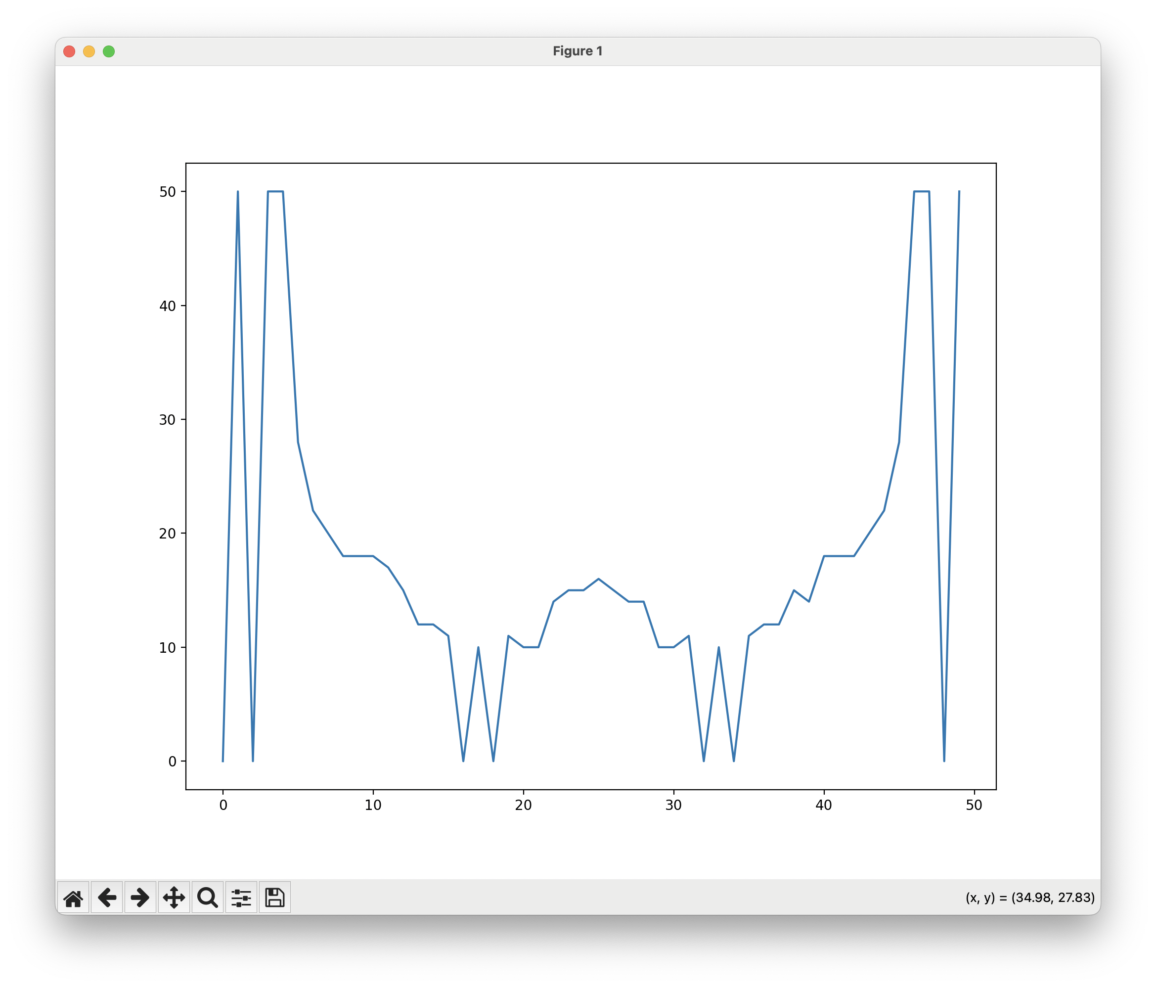 A mask that isn’t manufacturable because of rapid jogs.
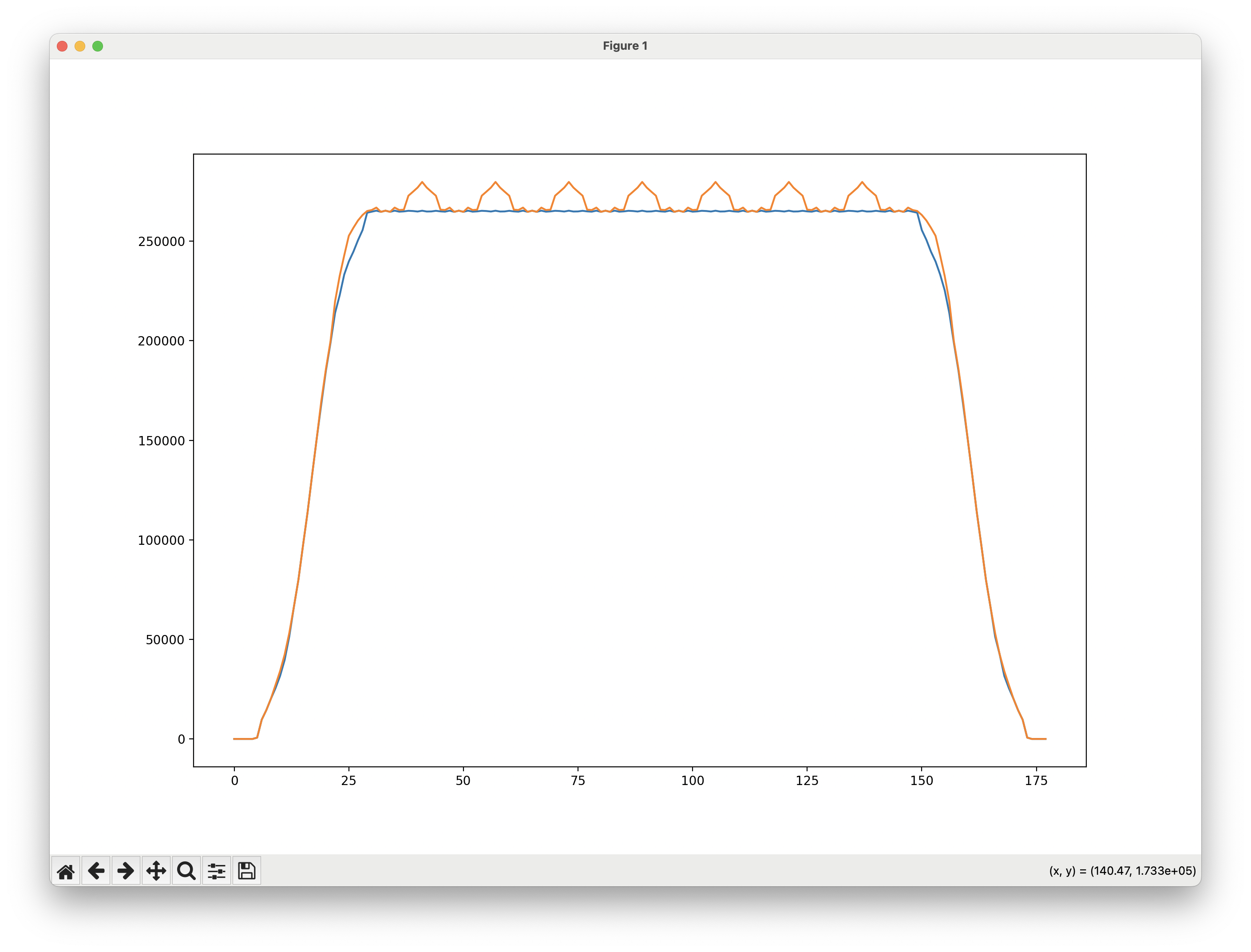 While the vampire mask isn’t feasible, it works computationally.
Some other failed candidates:
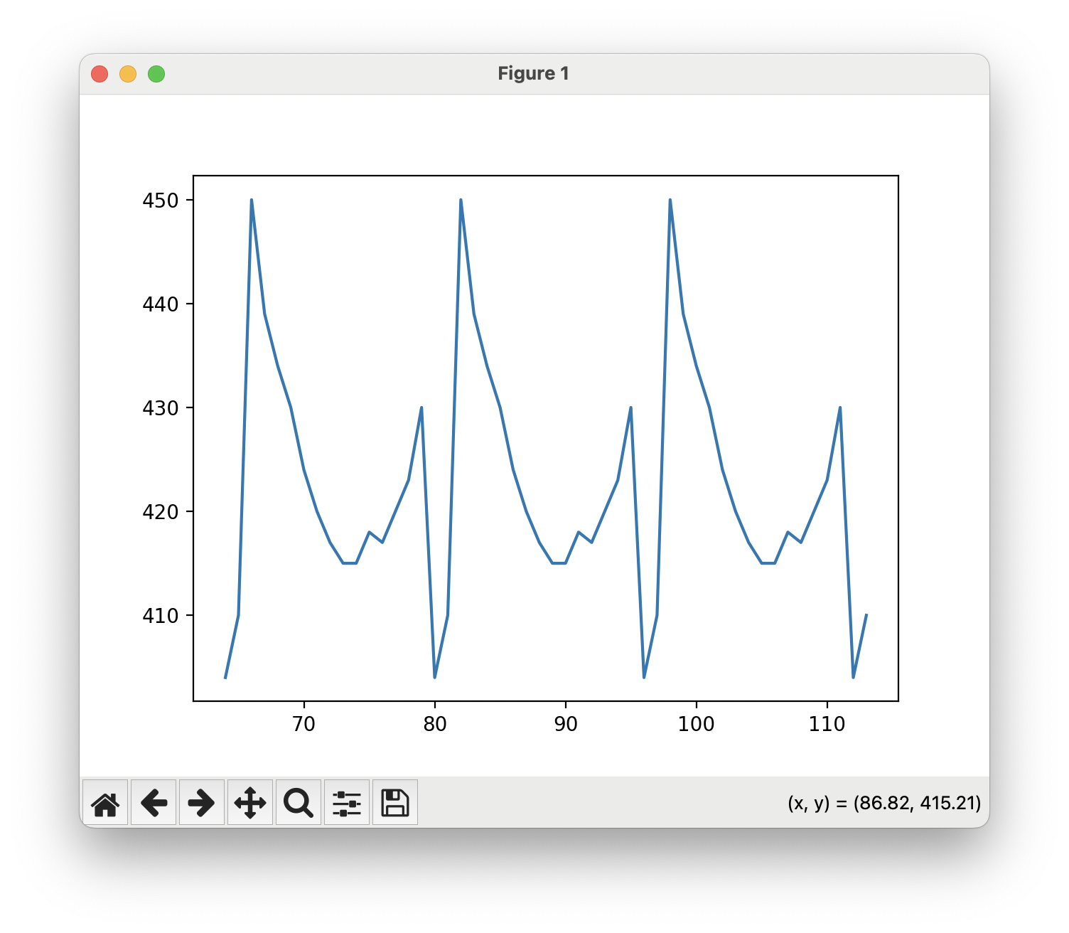 (This is actually duplicated three times in a row.)
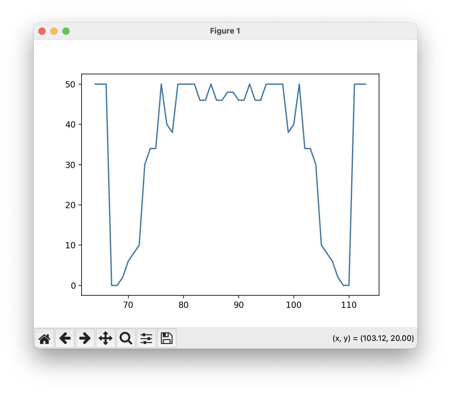
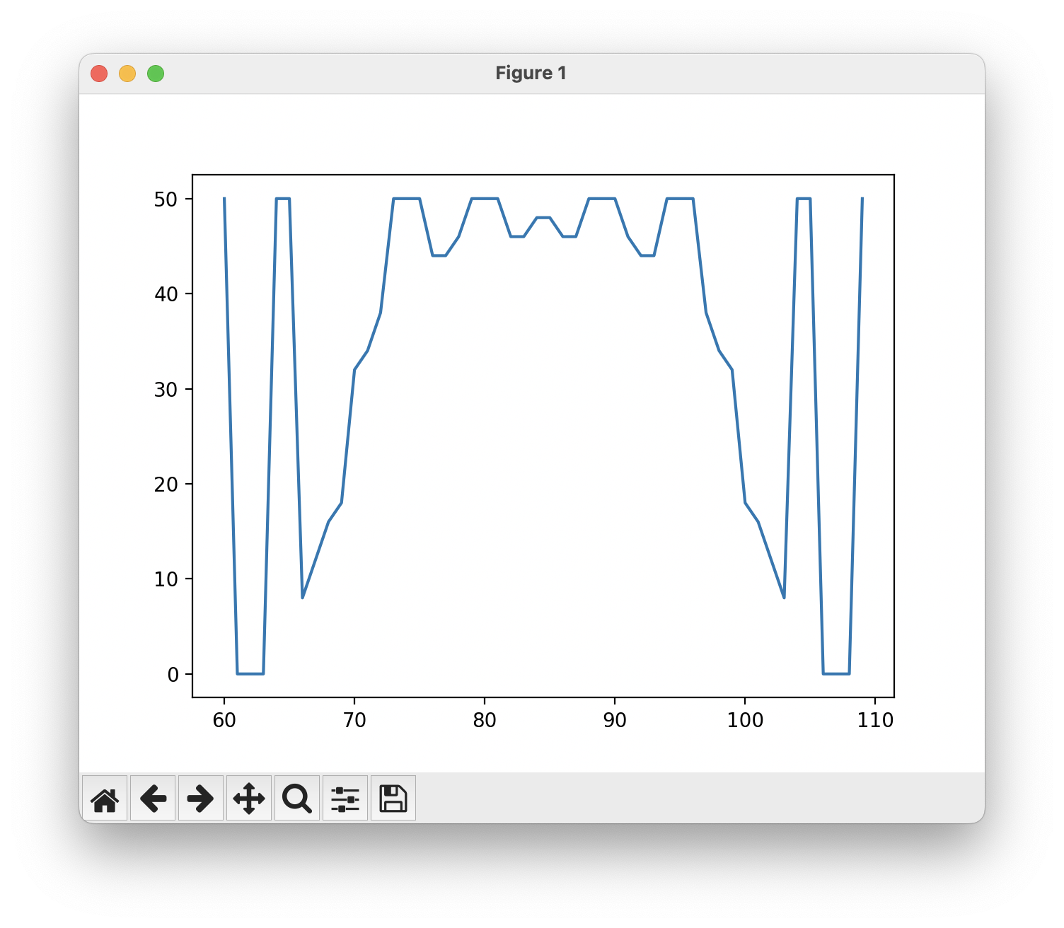
Some effort was put into a human-assisted search; with the cumulative exposure and an individual light profile graphed simultaneously, it is easy to see where and why the exposure becomes uneven. Selecting a column to nibble on by hand, and then asking the computer to do the nibbling until the error was trimmed produced a servicable mask. Ideally the process would be entirely synthetic–what is this AI age for even.
A Smoothness Heuristic (That Did Work)
A heuristic that did work is one that ensures the mask edge is relatively smooth. A slope-delta calculation compares the slope between pairs of cells at the forefront of the filter. Given a column i, the filter fronts for i-1 and i form the left slope, and the fronts for i and i + 1 form the right slope. The slope delta is the left slope minus the right slope. Cells at either end, which have only one neighbor, mirror their inner neighbor to the outside.
The heuristic used in the search has two conditions:
- the column must have some positive error to be considered in the search
- the column’s heuristic value is the slope delta

These rules keep the filter edge smooth, allowing the search to expand outwards to find the boundary made by the trim level. Cells that form valleys into the filter edge are prioritized for being filled in; cells that are smooth have a middling slope delta; cells that form mountains away from the filter edge are deprioritized. This enforces smoothness of the filter shape to make it manufacturable, while allowing some local conformance to error peaks. (This heuristic reminds me of surface tension; the edge creeps outwards, until it hits the error limit, and stops. Like surface tension, it is a physical property that acts between neighbors and creates a global trend.)
This heuristic produced a filter that successfully trims the cumulative exposure to 0.27% variation, while producing a manufacturable filter.
One additional detail is that the search worked better when the trim value was lowered past the minimum exposure level in the unfiltered strip, to 95%. After examination of the cumulative graph overlaid with the individual spots, this turned out to be because these minimum points prevented the mask from reaching deep enough into some areas, where more significant light levels are; they were outside the achievable slope rate of the filter.
This is what a filter looks like, along with the before-and-after simulations of the cumulative exposure.
 The winning mask. Note that the slopes at the edges are included for scale, and are outside of the light spot area.
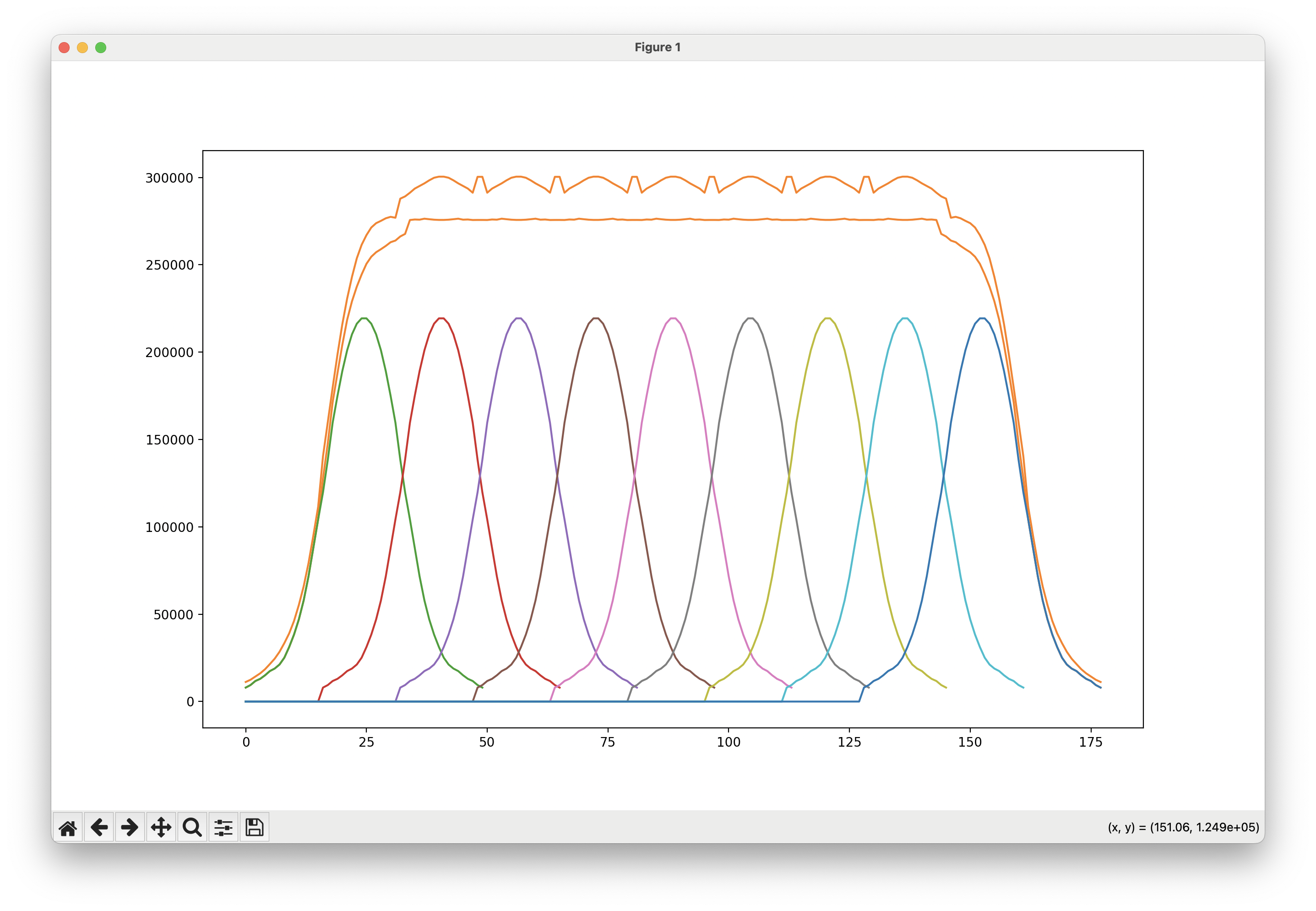 Individual light spots, their cumulative sum, and the filtered sum.
In practice, the edges will be smoothed and expanded; the sharp points represent a 1mm-wide cell area. This mask provides a good scaffolding for finding curves that cross partial cells and compensating for the sloped shapes of the light spots.